ImageJ, ImageJ2, and Fiji: What to Install to Start
ImageJ is an extensible image analysis program widely used in life sciences. Fiji is an ImageJ2 distribution that incorporates numerous plugins and libraries for scientific analysis; it also includes the original ImageJ, so many classic commands remain available.
Fiji bundles plugins and offers an integrated update and documentation mechanism. This does not make any installation equivalent to another: plugins, their versions, and local preferences can change the available commands. Record the version and relevant plugins when the procedure will support results that must be repeated or shared.
ImageJ does not determine by itself what an image represents or whether a method is suitable for a biological question. Segmentation and measurements depend on acquisition, sample type, and analytical decisions. This walkthrough serves to build an explicit and verifiable workflow, not to impose a universal threshold or replace method validation.
Installing Fiji and First Startup
Download Fiji from the official imagej.net downloads page and choose the package matching your operating system and architecture. The page distinguishes, among others, versions for Windows, macOS, and Linux, as well as x86-64 and arm64 architectures. Latest is the recommended option for most users; Stable is reserved for those needing Java 8 compatibility, older systems, or legacy plugins.
Fiji is distributed as a portable application: it is downloaded and extracted, without a traditional installer. On Windows, the project recommends saving it within a user folder and not in Program Files, because write permissions in that location can prevent Fiji from updating correctly. Open the application from the extracted folder and keep its files there so the updater can manage them.
Fiji Latest requirements include Windows 10 or later (x86-64 or arm64), macOS 11 or later (Apple Silicon or Intel), and Ubuntu 22.04 LTS or later (x86-64 or arm64). Other systems require a Java 21 environment; some plugins using native libraries may have limitations.
To maintain a coherent installation, update from the Fiji mechanism and restart when the program requests it. Avoid copying plugins randomly or keeping multiple copies of the same JAR file in plugins: Bio-Formats warns that duplicate versions can cause errors. If a plugin is essential for an analysis, record its name and version along with the protocol.
Opening Images with Bio-Formats and Checking Dimensions
Bio-Formats allows importing microscopy formats that ImageJ does not open by itself and presenting them as multidimensional images. In Fiji, open Plugins > Bio-Formats > Bio-Formats Importer and select the file; you can also drag it to the Bio-Formats shortcut. The import dialog allows choosing how to load the image and, depending on the files, grouping elements of a set into a structure with spatial and temporal dimensions.
When importing, check the selected series and the X, Y, channel, Z, and time dimensions. If data are spread across files with similar names, the Group files with similar names option can gather them into a single multidimensional image. Before using it, verify that the files belong to the same set and that the grouping reflects the intended order.
Review image information with Image > Show Info and, where applicable, Image > Properties. Check units, pixel size, Z depth, and time interval if those values are present. The included information depends on the format and acquisition file; if a reliable spatial scale is missing, do not interpret pixels as microns until calibrated with an appropriate reference. Opening an image with the importer also does not prove that all its properties have been preserved in a subsequent export.
A reproducible Fiji microscopy workflow
Follow these steps to keep the original image distinct from analysis outputs and make measurements interpretable.
-
1. Import
Select series and dimensions
-
2. Check calibration
Confirm units and scale
-
3. Preserve the original
Analyze a separate copy
-
4. Segment and review
Inspect masks and counting options
-
5. Measure and document
Keep settings with results
-
6. Export and check
Verify the saved file
Specific import options and analysis settings depend on the file, image, and research question; this sequence does not validate a segmentation method.
Creating a Working Copy and Distinguishing Display from Data
Keep the original file unmodified and perform the analysis on a working copy. The original serves as a reference to compare results and review applied transformations.
The Image > Adjust > Brightness/Contrast... controls normally change how intensity is represented on screen, without altering pixel values in 8, 16, or 32-bit grayscale images. In RGB images, brightness and contrast changes can modify pixels. Display and pixel values are not the same: check which one is being modified before measuring.
Type conversion can also change values. For example, converting a 16 or 32-bit image to 8 bits can rescale intensities according to the display range. To measure signal, work with appropriate intensity data and avoid converting the original just to facilitate its appearance. Separating channels with Image > Color > Split Channels can facilitate analysis, but keep the source image and document the channel used.
Process > Subtract Background... and filters can alter intensities and structures, so it is advisable to apply them on a copy and choose them according to the image type. Define and record the procedure before comparing groups. If the goal is to quantify intensities, measure on the corresponding intensity image, not on a binary mask created to locate objects.
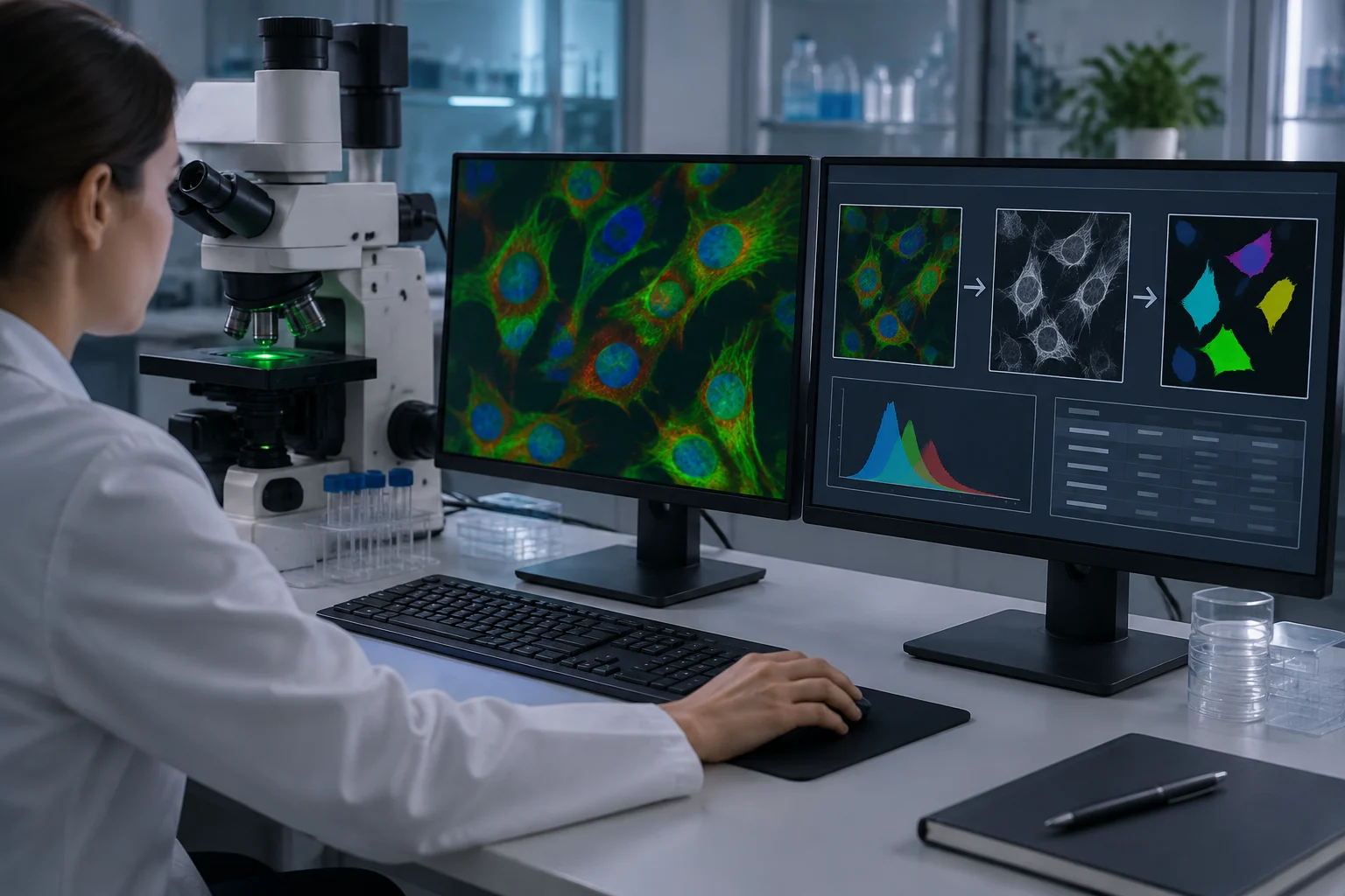
Segmenting and Counting Objects Without Fixing a Universal Threshold
The threshold converts an intensity image into a selection of pixels that the program treats as objects or background. Open Image > Adjust > Threshold..., inspect what remains marked, and adjust the method according to contrast and the analytical question. An automatic threshold does not validate segmentation: check that it includes the sought structures without incorporating relevant background and apply a consistent criterion to comparable images.
When segmentation is reasonable, use Apply or Process > Binary > Make Binary to create a working mask. The mask serves to delimit areas; it does not preserve the same intensity information as the original image. To count connected components, run Analyze > Analyze Particles... on the mask or thresholded image. Configure size range and circularity only if they respond to criteria defined for the experiment, and visually review the generated contours.
Analyze Particles offers options such as Exclude on Edges, Include Holes, contour visualization, and sending regions to ROI Manager. Each choice changes what is counted. Excluding objects touching the edge can be appropriate to avoid incomplete objects, but it also reduces the count of peripheral structures; including holes changes the measured area. Inspect exclusions and objects in representative images before processing a full series.
Process > Binary > Watershed can separate certain touching objects in a binary mask, but it does not resolve all overlap or identify cells by itself. If an object that biologically should remain united is split, the count is biased; if two real objects are not separated, the opposite occurs. Record if it was applied and with what criterion. A component count in a 2D projection is not, by itself, a volume measure or a cellular identification.
Calibrating Scale, Measuring Regions, and Saving ROIs
If the image contains a valid calibration, verify pixel size and unit before measuring. If not calibrated, use Analyze > Set Scale... with a known distance and a line drawn over a reference acquired under appropriate conditions. The tool assigns spatial units to measurements; a value entered without a reliable reference does not create a valid calibration. Check units and scale before reporting areas or lengths.
In Analyze > Set Measurements... select the necessary variables: area, mean, standard deviation, perimeter, centroid, or integrated density, among others. Analyze > Measure calculates values for the active selection. To measure intensity within a region, select the ROI on the original intensity image or intended channel; a mask delimits the region, but its binary pixels do not replace signal values.
ROI Manager allows saving and retrieving regions of interest. Add selections with Analyze > Tools > ROI Manager... and save the ROI set to link them with the corresponding sample and image. In a repeatable measurement, specify which channel is measured, how regions were defined, and whether edges or background areas were excluded. Area, intensity, and object count are distinct magnitudes and should not be exchanged as if they described the same result.
Analyze > Analyze Particles... can produce counts and measurements of each object, while the Set Measurements menu determines which columns are saved. Export the table from the Results window via File > Save As or the measurement command indicated by ImageJ. Keep the association between each row, the image, the ROI, and the channel or plane position; an isolated table, without those data, can lose context necessary for interpretation.
Exporting Results and Leaving a Reproducible Protocol
Save a working copy and the results table separately. ImageJ allows saving images in TIFF; to write with Bio-Formats use Plugins > Bio-Formats > Bio-Formats Exporter. File > Save As... is not equivalent to the Bio-Formats exporter: documentation warns that saving a TIFF via that route produces an ImageJ-specific TIFF, which other programs may not interpret in the same way. Check the exported file in the destination program when interoperability is important.
Bio-Formats offers export to compatible formats, including OME-TIFF. Select the exporter when you want to use Bio-Formats and confirm the file name and extension before saving. The extension may depend on the format chosen in the export dialog; do not assume that writing .ome.tif will automatically preserve expected properties. Keep the original acquisition file and the processed copy as separate elements.
To repeat a manual sequence, open Plugins > Macros > Record before executing commands and save the generated code. The Recorder helps record operations and parameters, although it does not replace documentation of the dataset, unrecorded options, or visual review of results. Record the Fiji version, relevant plugins, input files, analyzed channels, scale, threshold, filters, and Analyze Particles options.
Before closing the analysis, check this list:
- Keep the original and clearly mark processed copies.
- Review dimensions, metadata, and calibration before measuring.
- Separate display adjustments from operations that modify pixels.
- Inspect masks, edge exclusions, and object separation.
- Save tables, ROIs, and parameters that explain the result together.
- Export with the method corresponding to the format and confirm the file opens in the destination.